Normal Distributions, z Scores, and Transformations

Probability and the Normal Curve

Probability is the mathematical study of chance. Early applications of probability involved understanding games of chance, which can be viewed as repetitions of independent events. For example, if you flip a coin multiple times, each coin flip is independent of the previous one and next one. Similarly, if you roll a pair of dice repeatedly, each roll is independent of the previous one or next one. The chance that you will see heads on a single coin flip is always the same - .5 or 1 out of 2, because there are two possible outcomes and heads is one of those. If you flip a coin 10 times, however, you probably won't see exactly five heads - there may be six or four or even nine heads. It is possible, although unlikely with a fair coin, to see all 10 flips result in heads.

Consider another example to understand about probability. Suppose you are rolling a pair of dice repeatedly and adding up the dots on the top of each die. A die has six sides, numbered 1 to 6. Because you are adding two dice, the possible sums range between 2 (for snake-eyes - two 1s) and 12 (for box-cars - two 6s). Here is a table of the possible combinations of dice. The number appearing on the dice are indicated by the row and column labels and the sums are shown in each interior cell.

Values for Dice	1	2	3	4	5	6
1	2	3	4	5	6	7
2	3	4	5	6	7	8
3	4	5	6	7	8	9
4	5	6	7	8	9	10
5	6	7	8	9	10	11
6	7	8	9	10	11	12

There are 36 (6x6) possible outcomes, some of which result in the same sum. For example, a sum of 7 can occur six different ways. Notice that there is only one way to obtain a sum of 2 and one way for a 12. These are the least likely sums. The probability associated with each sum is the ratio of the number of ways it can occur divided by the total number of possibilities. For example, the probability of obtaining a sum of 3 is 2 out of 36 or .056 presenting 5.6% of the potential outcomes. What is the probability of obtaining a sum of 11, or 8, or 5? What sum is the most likely?

If you repeatedly rolled two dice many, many times and record the sums that you obtained, their frequencies would eventually resemble the pattern shown in the table. By counting the number of times 7 occurred, for example, and dividing that number by the number of rolls, you can calculate the relative frequency of a sum of 7. Over many repetitions of the dice roll, the relative frequencies get closer and closer to the theoretical probabilities. This is called the Law of Large Numbers.

Graphing the probabilities results in the following pattern. Instead of two dice, if you rolled three the pattern would begin to look more bell-shaped. The more dice involved, the closer the pattern gets to the normal (bell-shaped) curve. This is called the Central Limit Theorem. Seeing this phenomenon in the context of sampling and making inferences, especially when drawing a random sample from a population and calculating the mean for a variable many times independently, the shape of the resulting distribution of means will be resemble the normal curve. Learning about the properties of normal distributions is very important.

probability distribution for sum of three dice

Examples of Normal Distributions

There are actually infinitely many normal distributions - they differ by the value of their means and standard deviations. Here are some important properties of normal distributions:

The distribution is symmetric, which results in the mean, median, and mode all being equal.
The area under the plot of the distribution (i.e., area between the x-axis and the curve) equals 1, representing 100% when considered as relative frequencies.
The height of the curve approximates a relative frequency, but the area under any single point is 0.
The tails (left and right extremes) of the curve approach, not never touch, the x-axis (i.e., the tails are asymptotic to the x-axis).

Use of the Normal Distribution

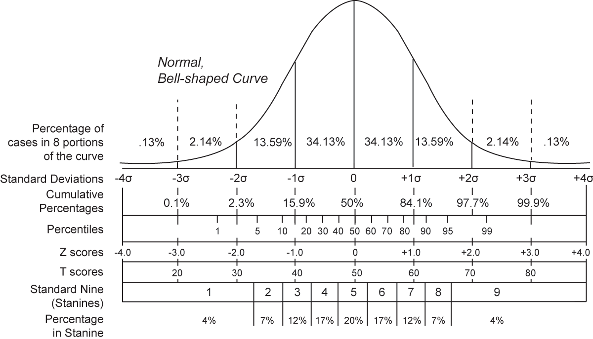
Any raw score from a normal distribution can be mapped onto a normal curve if the mean and standard deviation associated with the raw score is known. The graph below illustrates the mapping of several different types of scores. Notice that percentiles can be derived from the curve as well.

mapping of raw scores and others to normal curve

mapping of raw scores and others to normal curve

Notice that approximately 68% of the cases are within one standard deviation of the mean, 95% are within two standard deviations, and over 99% are within three standard deviations.

The Standard Normal Distribution

Even though there are many normal distributions, one of those has been designated to be the "standard" normal distribution. The standard normal distribution is the normal distribution with a mean of 0 and a standard deviation of 1. Notice the line labeled Z scores in the graph above. Compare this line to the line labeled Standard Deviations just below the x-axis. Notice that a z score of +1.0 corresponds to a point under the curve labeled +1σ. Any raw score can be converted to a z score and back using these formulas:

z = (X - X) / s

and

X = s * z + X

where X is the mean of the distribution of raw scores and s is the standard deviation of the distribution of raw scores.

Here is an example of how to use the conversion formulas:

Suppose you have a score of 15 on a test where the mean was 10 and the standard deviation was 2.5. The z score equivalent to a raw score of 15 is

z = (15 - 10) / 2.5 = 5 / 2.5 = 2

Another way to describe this score is that it is 2 standard deviations above the mean. In a normal distribution, a score of raw score of 15 would be higher than 97.7% of the other scores. Look at the graph above to locate the source of 97.7%.

Here is a related example. Suppose you wanted to provide extra help to anyone who scored more than one standard deviation below the mean. What raw scores should you look for? Scoring one standard deviation below the mean results in a z score of -1. To determine the associated raw score, use the second conversion formula

X = 2.5 * (-1) + 10 = -2.5 + 10 = 7.5

Anyone scoring 7.5 or lower would be offered extra help. By inspecting the graph above, can you determine what percentage of scores this would represent?

Converting to z scores allows raw scores from different testing situations to be compared. For example, which is better a 20 in Ms. Chan's class where the mean was 12 and the standard deviation was 6, or a 15 in Mr. Williams' class where the mean was also 12 but the standard deviation was 2? Let's compare the z scores.

z_c = (20 - 12) / 6 = 8 / 6 = 1.3

z_w = (15 - 12) / 2 = 3 / 2 = 1.5

The 15 in Mr. Williams' class is better than the 20 in Ms. Chan's class, by .2 standard deviations.

Visit this site (http://psych.colorado.edu/~mcclella/java/normal/normz.html) to use an applet that will convert a raw score, with its associated mean and standard deviation, to a z score. This site (http://davidmlane.com/hyperstat/z_table.html) calculates the area under the curve for different z values and intervals.

Other Transformations

Converting raw scores to z scores involves to mathematical operations, adding/subtracting and multiplying/dividing. Instead of converting raw scores to z scores, raw scores can be converted into other types of scores. This process is called transformation. Here are some general guidelines about the effects of different transformations on distributions and their means and standard deviations.

Type of Transformation	Effect on the Distribution	Effect on the Mean	Effect on the Standard Deviation
Adding a positive number	Shifts it to the right	Increases it	No effect
Subtracting a positive number	Shifts it to the left	Decreases it	No effect
Multiplying a positive number	Stretches it	Multiplies it	Increases it
Dividing a positive number	Shrinks it	Divides it	Decreases it